The Sharpe Ratio is a measure of the risk-adjusted return on an investment. It was created by William F. Sharpe. The Ratio takes into account three values, a. Expected return on an investment/Past returns, b. The risk-free rate of return and c. Standard deviation of the investment’s return (volatility). The Sharpe Ratio is as follows:

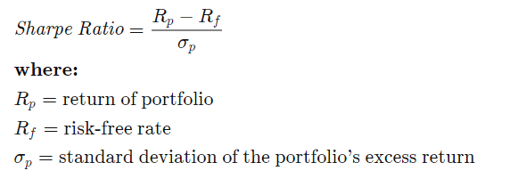
Understanding the Sharpe Ratio 

The higher the Sharpe Ratio, the better its risk-adjusted performance. This can be influenced in two ways. Firstly, it can be increased with a larger value of excess returns. Secondly, a smaller standard deviation (or lower volatility) can increase the Sharpe Ratio as well.

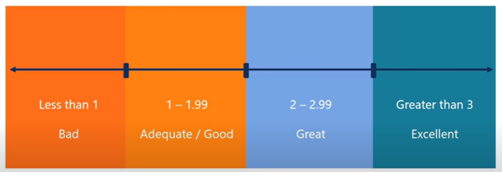
Now, what is a good Sharpe Ratio?

1. A Sharpe Ratio of <1.0 is considered bad
2. A Sharpe Ratio between 1 – 1.99 is adequate
3. A Sharpe Ratio between 2-2.99 is great
4. Lastly, a Sharpe ratio >=3 is excellent

It can be also thought that the Sharpe Ratio is the number of standard deviations by which the portfolio’s return must fall in order to underperform the risk-free investment. Sharpe Ratio is more relevant when compared to the Sharpe Ratios of other portfolio ‘sharpes’. You can think of it as a PE ratio where it is not very useful on a standalone basis but good as a comparison tool with other investments.

Limitations of Sharpe Ratio

However, there are some limitations of the Sharpe Ratio. 

Firstly, one limitation of the Sharpe Ratio is that it is typically based on historical returns. Hence, there is an assumption that the historical returns will provide a good gauge of the investment’s future returns (However, this may not hold through as past results are not reflective of future performance).

Secondly, the Sharpe Ratio can be manipulated by changing the time period of the investment. For example, the time period can be extended to include years of superior returns. Furthermore, a longer time period tends to result in a lower estimate of volatility than longer periods.

In addition, the Sharpe Ratio assumes that returns are normally distributed. However in reality investment returns rarely follow a normal distribution. Rather, they tend to have high peaks and a fat tail. This is because the returns distribution might suffer from kurtosis.

Lastly, the Sharpe Ratio only takes into account the magnitude but not the direction of volatility. As you know, volatility can work for and against investors depending on its direction. Hence, the Sharpe Ratio may penalise investments with a large upside deviation but small pullbacks (or downside deviation). This limitation can be countered by the Sortino Ratio which I will discuss in the later section.

Getting the data for Sharpe Ratio

Now, how do we get the data for the Sharpe Ratio? Let us begin with the return on investment. As it is difficult to figure out the investment’s expected return, it will be easier to use the investment’s past returns data. This can be found on the investment’s information page, or financial websites such as Yahoo Finance. While the investment’s information page provides returns data for specific intervals (e.g. YTD, 1 month, 1 yr and so on), you can find a specific interval using the financial sites.

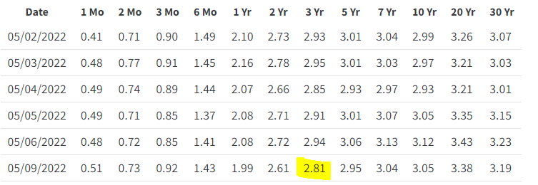
Next, how do we get the risk-free rate of return? This can be done by using the treasury bills yields. To find the T-bills rates for a specific period, you can get the data from the U.S. Treasury Department Website.

Lastly, we can find the standard deviation of the investment via their information page. Additionally, this can be found on financial sites such as Yahoo Finance (under ‘risk’). However, for the standard deviation, data provided is typically done for regular time periods. Hence our calculations for the Sharpe Ratio would be based on the respective time periods as well.

Example

Now that we know how to get the data to calculate the Sharpe Ratio, we will do an example with two exchange-traded funds (ETFs), ISAC and IWDA. Both ISAC and IWDA are Irish-Domiciled ETFs, but ISAC tracks the MSCI ACWI Index for both developed and emerging markets exposure. IWDA tracks the MSCI World Index for developed market exposure. For the purpose of this example we will be using a 3Y time period. For the 3-year time period, the Treasury Bill Yield is 2.81%.

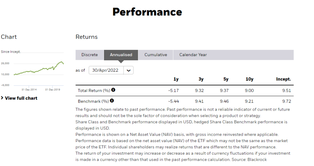
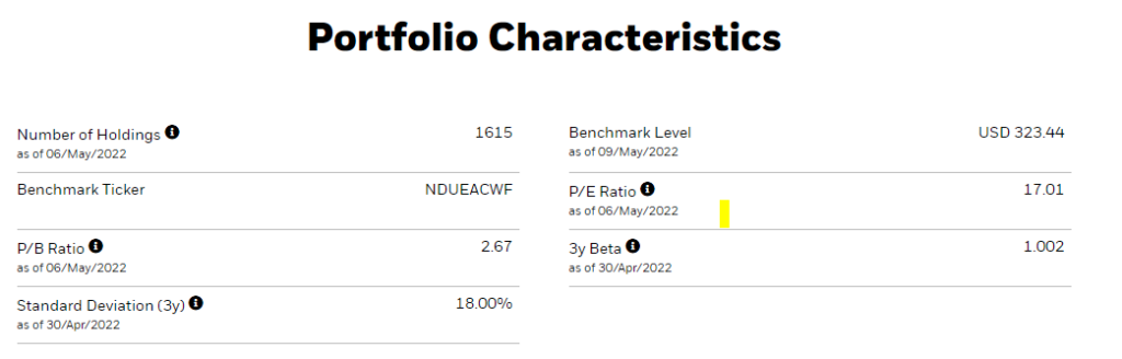
Firstly, we will calculate ISAC’s Sharpe Ratio. From the website, it states the following data:

1. Past Annualised Return (3Y): 9.32%
2. 3-year Treasury Bill Yield: 2.81%
3. Standard Deviation (3Y): 18.00%

Using the Sharpe Ratio formula, we get a Sharpe Ratio of 9.32 – 2.81 / 18 = 0.362. 

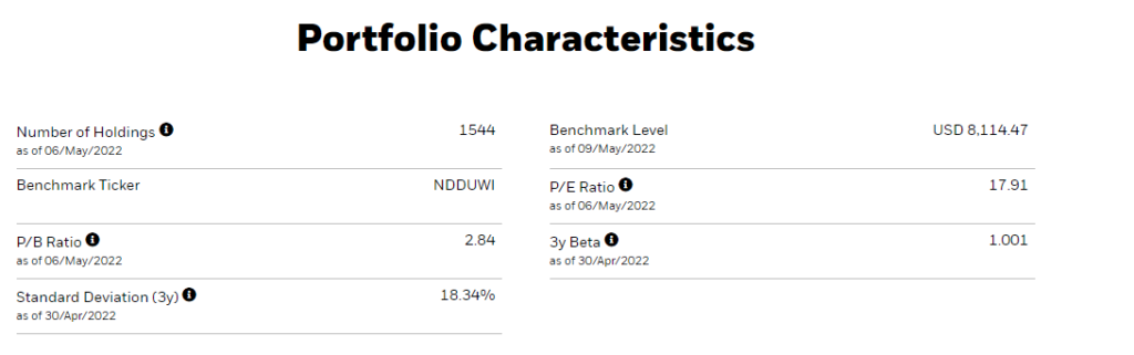
Now moving on to IWDA, the data required is as follows:

1. Past Annualised Return (3Y): 10.50%
2. 3-year Treasury Bill Yield: 2.81%
3. Standard Deviation (3Y): 18.34%

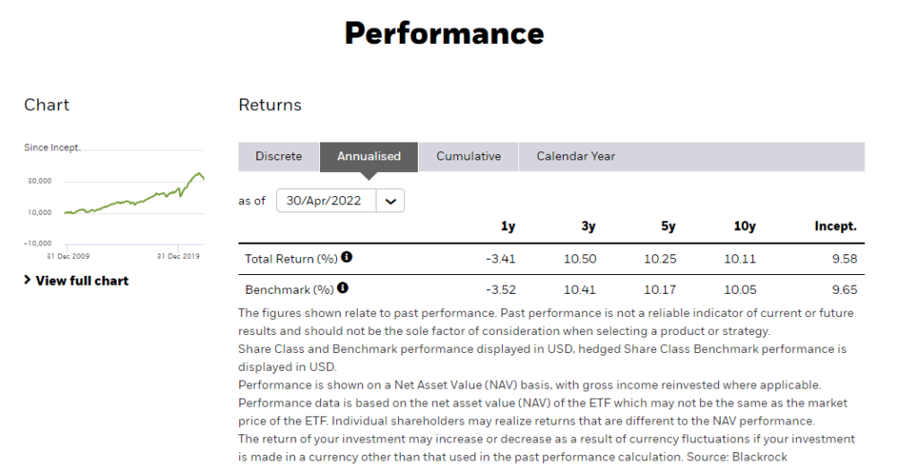
Using the formula we get a Sharpe Ratio of 0.419. Based on the Sharpe Ratio, IWDA can be considered a better investment ‘portfolio’ than ISAC when accounting for risk-adjusted returns. However, both investments may be deemed as poor investments as their Sharpe Ratio is under 1.

[A possible reason for ISAC to have a lower ratio than IWDA would be their exposure to developing markets which fared poorly in 2021. In addition, given the high volatility in the past few years, both assets Sharpe Ratio is lower than compared to longer time horizons]

Sortino Ratio

A variant of the Sharpe Ratio, the Sortino Ratio differentiates harmful volatility from overall volatility. While the Sharpe Ratio uses overall volatility (or standard deviation), the Sortino Ratio uses the downside volatility (or standard deviation of the downside instead). In other words, the Sortino Ratio is a measure of the performance of an investment relative to its downside deviation. The Sortino Ratio formula is as follows.

Just like the Sharpe Ratio, the higher the ratio, the better the investment is. I won’t dive more into the Sortino Ratio, but if you would like me to go through it in the future, do let me know in the comments below : )

Conclusion

And there we have it! Hopefully, this article will help you understand the Sharpe Ratio, and how it can be a useful tool in calculating an investment’s risk-adjusted return. Do let me know what other content you would like me to cover in the future.

Cheers!

-Rice

Useful Resources

Do check out some of the useful resources that I referenced in the article as well! They do offer more insights to the Sharpe Ratio.

Website:

1. Sharpe Ratio
2. Sortino Ratio

• Instagram
• Reddit
• Medium
• Mail
• WordPress